Initialize:
pi = 0.500000, mu_1 = -1.804556, mu_2 = 1.299319, sigma_1 = 2.170121, sigma_2 = 2.170121
Iteration 1:
pi = 0.513579, mu_1 = -1.452977, mu_2 = 1.021019, sigma_1 = 1.508890, sigma_2 = 2.027382
Iteration 2:
pi = 0.511131, mu_1 = -1.649551, mu_2 = 1.214156, sigma_1 = 1.223416, sigma_2 = 1.962810
Iteration 3:
pi = 0.510756, mu_1 = -1.864417, mu_2 = 1.436274, sigma_1 = 0.898038, sigma_2 = 1.787585
Iteration 4:
pi = 0.523272, mu_1 = -1.985462, mu_2 = 1.655792, sigma_1 = 0.685328, sigma_2 = 1.549351
Iteration 5:
pi = 0.539953, mu_1 = -2.014110, mu_2 = 1.821443, sigma_1 = 0.636488, sigma_2 = 1.338752
Iteration 6:
pi = 0.554587, mu_1 = -2.004785, mu_2 = 1.935851, sigma_1 = 0.636896, sigma_2 = 1.195700
Iteration 7:
pi = 0.564860, mu_1 = -1.988832, mu_2 = 2.008172, sigma_1 = 0.646324, sigma_2 = 1.108705
Iteration 8:
pi = 0.570641, mu_1 = -1.977248, mu_2 = 2.046598, sigma_1 = 0.655227, sigma_2 = 1.063504
Iteration 9:
pi = 0.573534, mu_1 = -1.970567, mu_2 = 2.064913, sigma_1 = 0.661230, sigma_2 = 1.042708
Iteration 10:
pi = 0.574914, mu_1 = -1.967120, mu_2 = 2.073345, sigma_1 = 0.664600, sigma_2 = 1.033444
Iteration 11:
pi = 0.575559, mu_1 = -1.965440, mu_2 = 2.077213, sigma_1 = 0.666314, sigma_2 = 1.029282
Iteration 12:
pi = 0.575860, mu_1 = -1.964643, mu_2 = 2.078994, sigma_1 = 0.667143, sigma_2 = 1.027388
Iteration 13:
pi = 0.575999, mu_1 = -1.964270, mu_2 = 2.079815, sigma_1 = 0.667534, sigma_2 = 1.026519
Iteration 14:
pi = 0.576063, mu_1 = -1.964097, mu_2 = 2.080195, sigma_1 = 0.667718, sigma_2 = 1.026118
Iteration 15:
pi = 0.576093, mu_1 = -1.964016, mu_2 = 2.080371, sigma_1 = 0.667803, sigma_2 = 1.025933
Iteration 16:
pi = 0.576107, mu_1 = -1.963979, mu_2 = 2.080452, sigma_1 = 0.667842, sigma_2 = 1.025848
Iteration 17:
pi = 0.576114, mu_1 = -1.963962, mu_2 = 2.080490, sigma_1 = 0.667861, sigma_2 = 1.025808
Iteration 18:
pi = 0.576117, mu_1 = -1.963954, mu_2 = 2.080507, sigma_1 = 0.667869, sigma_2 = 1.025790
Iteration 19:
pi = 0.576118, mu_1 = -1.963950, mu_2 = 2.080516, sigma_1 = 0.667873, sigma_2 = 1.025781
Iteration 20:
pi = 0.576119, mu_1 = -1.963948, mu_2 = 2.080519, sigma_1 = 0.667875, sigma_2 = 1.025777The EM Algorithm — Example and Theory
2025-10-28
The EM Algorithm
- example
- bit more theoretical
Example: Two-component Gaussian mixture
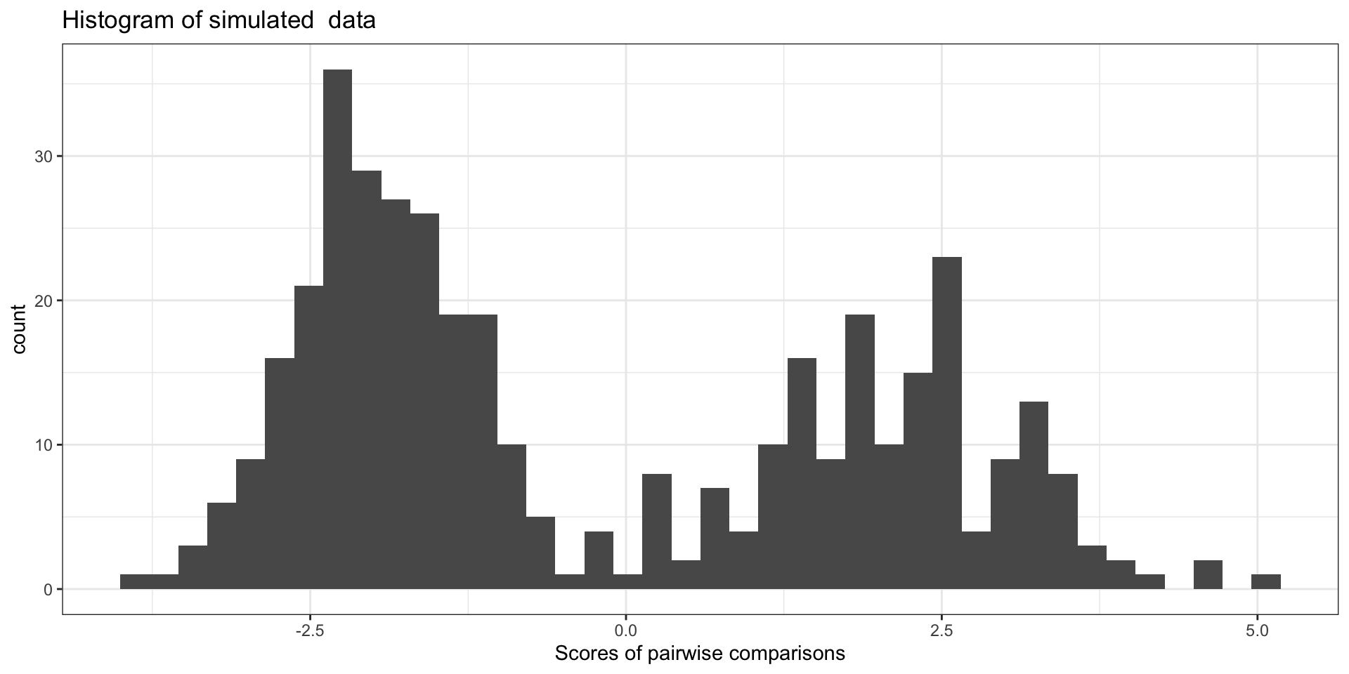
The scores we observe from pairwise comparisons of data from two sources seems to come from two (normal?) distributions:
Model Assumption
We assume that the underlying model is
\[ X_i \sim \pi\,N(\mu_1,\sigma_1^2) + (1-\pi)\,N(\mu_2,\sigma_2^2),\quad i=1,\dots,n. \]
Here the latent variable is the component indicator \(Z_i\in\{1,2\}\) with
\[P(Z_i=1)=\pi,\quad P(Z_i=2)=1-\pi.\]
Unfortunately, \(Z_i\) is not observed.
Model Parameters
A two-component model has parameters
\(\theta=(\pi,\mu_1,\mu_2,\sigma_1^2,\sigma_2^2)\).
If the labels \(Z_i\) were observed, parameter estimation would be straightforward.
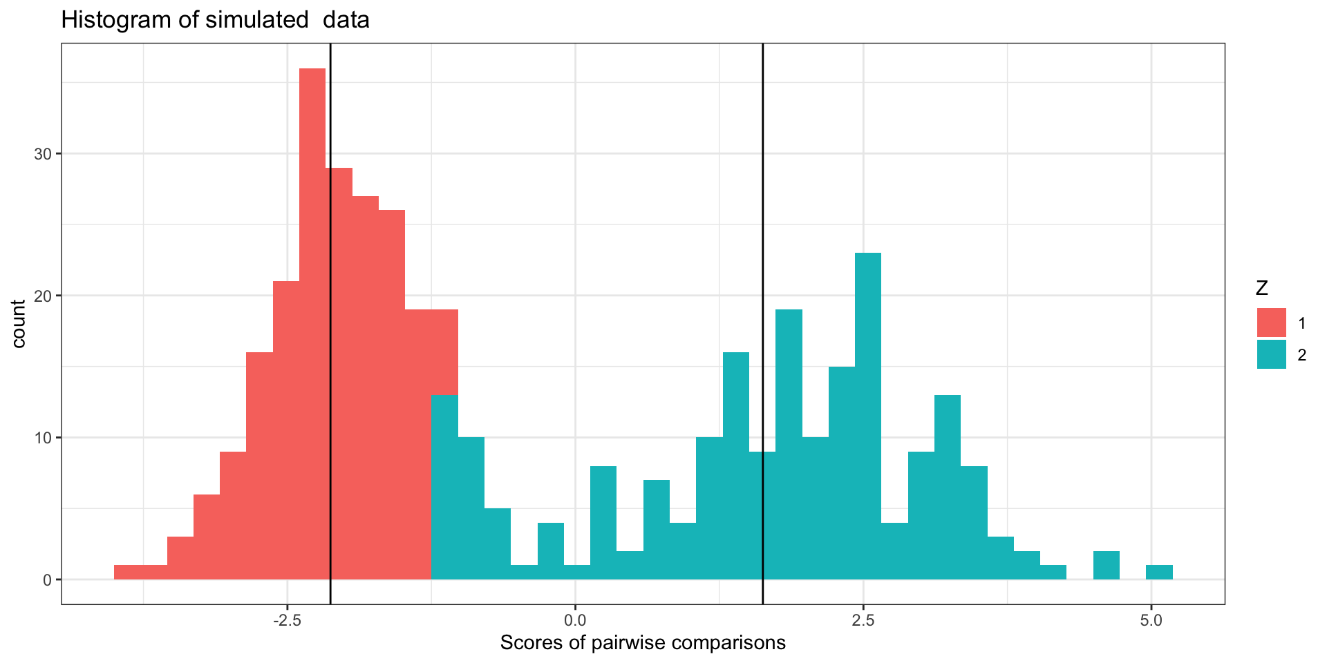
Since \(Z_i\) is not observed, we use some heuristics to get started:
\(\mu_1 < \mu_2\) (we will assume that \(Z=1\) will translate to ‘not a match’ and \(Z=2\) will be ‘match’)
\(\pi^{(1)} = 1/2\);
\(\mu_1^{(1)}, \mu_2^{(1)}\) means of lower and upper halves of scores; \(\sigma_1^{(1)}, \sigma_2^{(1)}\) sds of lower and upper half
Initial Step
Expectation Step
Based on estimate \({\hat\theta}^{(t)}\), we calculate the probabilities:
\[ P(Z_i=1\mid x_i,\theta^{(t)}) = \frac{\pi^{(t)}\,\phi(x_i;\mu_1^{(t)},\sigma_1^{2(t)})}{\sum_{k=1}^2 \pi_k^{(t)}\,\phi(x_i;\mu_k^{(t)},\sigma_k^{2(t)})} \] and
\[ P(Z_i=2\mid x_i,\theta^{(t)}) = \frac{(1- \pi^{(t)})\,\phi(x_i;\mu_2^{(t)},\sigma_2^{2(t)})}{\sum_{k=1}^2 \pi_k^{(t)}\,\phi(x_i;\mu_k^{(t)},\sigma_k^{2(t)})} \]
Maximization step
We get updated values \({\hat\theta}^{(t+1)}\) as
\[ \mu_k^{(t+1)} = \frac{\sum_i k \cdot P(Z_i = k \mid x_i,\theta^{(t)})}{\sum_i P(Z_i = k \mid x_i,\theta^{(t)})} \] \[ \sigma_k^{(t+1)} = \frac{\sum_i (x_i - \mu_j^{(t)})^2 \cdot P(Z_i = k \mid x_i,\theta^{(t)})}{\sum_i P(Z_i = k \mid x_i,\theta^{(t)})} \] \[ \pi^{(t+1)} = \frac{1}{n}\sum_i P(Z_i = 1 \mid x_i,\theta^{(t)}) \]
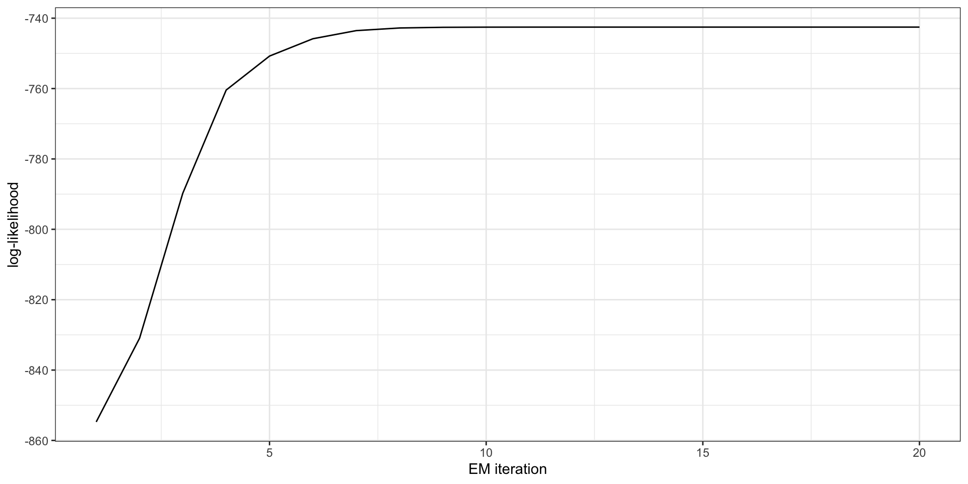
Run until convergence
Iteration 5:
pi = 0.539953, mu_1 = -2.014110, mu_2 = 1.821443, sigma_1 = 0.636488, sigma_2 = 1.338752
Iteration 6:
pi = 0.554587, mu_1 = -2.004785, mu_2 = 1.935851, sigma_1 = 0.636896, sigma_2 = 1.195700
Iteration 7:
pi = 0.564860, mu_1 = -1.988832, mu_2 = 2.008172, sigma_1 = 0.646324, sigma_2 = 1.108705
Iteration 8:
pi = 0.570641, mu_1 = -1.977248, mu_2 = 2.046598, sigma_1 = 0.655227, sigma_2 = 1.063504
Iteration 9:
pi = 0.573534, mu_1 = -1.970567, mu_2 = 2.064913, sigma_1 = 0.661230, sigma_2 = 1.042708
Iteration 10:
pi = 0.574914, mu_1 = -1.967120, mu_2 = 2.073345, sigma_1 = 0.664600, sigma_2 = 1.033444
Iteration 11:
pi = 0.575559, mu_1 = -1.965440, mu_2 = 2.077213, sigma_1 = 0.666314, sigma_2 = 1.029282
Iteration 12:
pi = 0.575860, mu_1 = -1.964643, mu_2 = 2.078994, sigma_1 = 0.667143, sigma_2 = 1.027388
Iteration 13:
pi = 0.575999, mu_1 = -1.964270, mu_2 = 2.079815, sigma_1 = 0.667534, sigma_2 = 1.026519
Iteration 14:
pi = 0.576063, mu_1 = -1.964097, mu_2 = 2.080195, sigma_1 = 0.667718, sigma_2 = 1.026118Iteration 15:
pi = 0.576093, mu_1 = -1.964016, mu_2 = 2.080371, sigma_1 = 0.667803, sigma_2 = 1.025933
Iteration 16:
pi = 0.576107, mu_1 = -1.963979, mu_2 = 2.080452, sigma_1 = 0.667842, sigma_2 = 1.025848
Iteration 17:
pi = 0.576114, mu_1 = -1.963962, mu_2 = 2.080490, sigma_1 = 0.667861, sigma_2 = 1.025808
Iteration 18:
pi = 0.576117, mu_1 = -1.963954, mu_2 = 2.080507, sigma_1 = 0.667869, sigma_2 = 1.025790
Iteration 19:
pi = 0.576118, mu_1 = -1.963950, mu_2 = 2.080516, sigma_1 = 0.667873, sigma_2 = 1.025781
Iteration 20:
pi = 0.576119, mu_1 = -1.963948, mu_2 = 2.080519, sigma_1 = 0.667875, sigma_2 = 1.025777Results
\(\hat{\pi} =\) 0.5761186
\(\hat\mu_1 =\) -1.9639484, \(\hat\mu_2 =\) 2.0805192
\(\hat\sigma_1 =\) 0.6678748, \(\hat\sigma_2 =\) 1.0257773
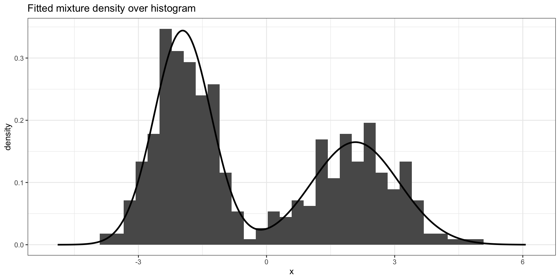
Inspect fitted mixture
Statistical Foundation of EM Algorithm
Let the observed data be \(X = (X_1,\dots,X_n)\) and let the latent (missing) data be \(Z = (Z_1,\dots,Z_n)\). The complete-data log-likelihood is
\[ \ell_c(\theta) = \log p(X,Z\mid\theta), \]
while the observed-data log-likelihood is
\[ \ell_o(\theta) = \log p(X\mid\theta) = \log \int p(X,Z\mid\theta)\,dZ.\]
Direct maximization of \(\ell_o(\theta)\) is often difficult.
E-step and M-step (concept)
EM constructs an iterative scheme. Given current parameter value \(\theta^{(t)}\):
E-step: compute the expected complete-data log-likelihood under the conditional distribution of the missing data given observed data and current parameters:
M-step: choose the next iterate as maximum of this expected complete-data log-likelihood
E-step and M-step (formula)
Iterate until convergence
- E-step:
\[ Q(\theta\mid\theta^{(t)}) = E_{Z\mid X,\theta^{(t)}}\left[ \ell_c(\theta) \right]. \]
- M-step:
\[ \theta^{(t+1)} = \arg\max_{\theta} Q(\theta\mid\theta^{(t)}). \]
Why does EM work?
For any \(\theta\) and \(\theta^{(t)}\):
\[ \ell_o(\theta) - \ell_o(\theta^{(t)}) = \log\frac{p(X\mid\theta)}{p(X\mid\theta^{(t)})} = \log E_{Z\mid X,\theta^{(t)}}\left[ \frac{p(X,Z\mid\theta)}{p(X,Z\mid\theta^{(t)})} \right]. \]
Using Jensen’s inquality, \(\log E[W] \ge E[\log W]\). Rearranging yields
\[ \ell_o(\theta) \ge Q(\theta\mid\theta^{(t)}) - H(\theta^{(t)}), \]
where \(H(\theta^{(t)}) = E_{Z\mid X,\theta^{(t)}}[\log p(Z\mid X,\theta^{(t)})]\) does not depend on \(\theta\).
Why does EM work? (2)
Choosing \(\theta = \theta^{(t+1)}\) that maximizes \(Q\) ensures
\[ \ell_o(\theta^{(t+1)}) \ge \ell_o(\theta^{(t)}), \]
so the observed-data log-likelihood is non-decreasing across iterations.
Convergence properties and limitations
- Monotonicity: EM never decreases the observed-data log-likelihood.
- Fixed points: Any limit point of EM is a stationary point (often a local maximum or saddle point) of the observed-data log-likelihood. EM can converge to local maxima.
- Speed: EM can be slow near the maximum — it typically has linear convergence.
- Identifiability: For mixture models, label switching means component labels are not identifiable — EM will converge to one labeling.
Practical tips and diagnostics
- Initialize EM multiple times with different random starts to avoid poor local maxima.
- Monitor the observed log-likelihood; watch for plateaus.
- Plot fitted densities to check fit.
- For mixtures, consider penalized likelihoods or Bayesian approaches to handle overfitting and component proliferation.
References
- Dempster, A. P., Laird, N. M., & Rubin, D. B. (1977). Maximum likelihood from incomplete data via the EM algorithm. Journal of the Royal Statistical Society: Series B (Methodological).
- McLachlan, G., & Peel, D. (2000). Finite Mixture Models. Wiley.
- Bishop, C. M. (2006). Pattern Recognition and Machine Learning — Chapter 9 (mixture models and EM).
